Since the 2010 election, pre-poll voting has been made easier. A new category of pre-poll vote was created for the 2010 election: the ordinary pre-poll vote, which is made within a voter's normal electorate. These ordinary pre-poll votes are counted on election night. Declaration pre-poll votes - which since 2010 are cast outside of a person's home electorate - are counted after the election night.
Prior to 2010, all pre-poll votes were treated as declaration pre-poll votes. Pre-poll voters had to provide a good reason to pre-poll (such as living too far from a polling booth). Since 2010, pre-poll voters simply need to declare that they won't be able to make it to a polling booth on election day.
In this analysis, I compare the vote outcomes for each seat and each vote-type with the on-election-day ordinary votes. Similar conclusions hold ...
- Absent voters in a seat typically do not favour the Coalition (when compared with on-election-day ordinary voters)
- Postal voters in a seat typically favour the Coalition (when compared with on-election-day ordinary voters)
- Pre-poll ordinary voters in a seat typically favour the Coalition (when compared with on-election-day ordinary voters)
- Pre-poll declaration voters in a seat typically favour the Coalition (when compared with on-election-day ordinary voters)
- Provisional voters in a seat do not typically favour the Coalition (when compared with on-election-day ordinary voters)
The charts, this time sorted by vote type, follow ...
Absent Votes


Postal Votes


Pre-poll Ordinary Votes


Pre-poll Declaration Votes


Provisional Votes


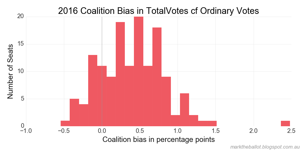
Total Votes


Counts and Proportions by Vote Type


Code
For the curious (and to help ensure I have not made a doozy of an error), my python code for the above charts follows. The data comes straight from the Australian Electoral Commission.import pandas as pd
import numpy as np
import matplotlib.pyplot as plt
plt.style.use('../bin/markgraph.mplstyle')
# --- get data
e2016 = pd.read_csv('./Data/HouseTcpByCandidateByVoteTypeDownload-20499.csv',
header=1, index_col=None, quotechar='"',sep=',', na_values = ['na', '-', '.', ''])
e2013 = pd.read_csv('./Data/HouseTcpByCandidateByVoteTypeDownload-17496.csv',
header=1, index_col=None, quotechar='"',sep=',', na_values = ['na', '-', '.', ''])
e2010 = pd.read_csv('./Data/HouseTcpByCandidateByVoteTypeDownload-15508.csv',
header=1, index_col=None, quotechar='"',sep=',', na_values = ['na', '-', '.', ''])
o2016 = pd.read_csv('./Data/HouseTcpByCandidateByPollingPlaceDownload-20499.csv',
header=1, index_col=None, quotechar='"',sep=',', na_values = ['na', '-', '.', ''])
o2013 = pd.read_csv('./Data/HouseTcpByCandidateByPollingPlaceDownload-17496.csv',
header=1, index_col=None, quotechar='"',sep=',', na_values = ['na', '-', '.', ''])
o2010 = pd.read_csv('./Data/HouseTcpByCandidateByPollingPlaceDownload-15508.csv',
header=1, index_col=None, quotechar='"',sep=',', na_values = ['na', '-', '.', ''])
# --- some useful frames
years = [2010, 2013, 2016]
data_year_all = zip([e2010, e2013, e2016], [o2010, o2013, o2016], years)
vote_types = ['OrdinaryVotesAdj', 'AbsentVotes', 'ProvisionalVotes',
'PrepollOrdinaryVotes', 'PrePollVotes', 'PostalVotes','TotalVotes']
vote_names = ['Ordinary Votes', 'Absent Votes', 'Provisional Votes',
'Pre-poll Ordinary Votes', 'Pre-poll Declaration Votes', 'Postal Votes','Total Votes']
type_names = zip(vote_types, vote_names)
Coalition = ['LP', 'NP', 'CLP', 'LNQ', 'LNP']
Labor = ['ALP']
Other = ['IND', 'GRN', 'KAP', 'ON', 'XEN', 'PUP']
# --- now let's calculate and plot the comparisons
totals = pd.DataFrame()
for all, ords, year in data_year_all:
all = all.copy() # let's be non-destructive
ords = ords.copy() # let's be non-destructive
print(year)
# re-label parties
def grouper(df):
df['PartyGroup'] = None
df['PartyGroup'] = df['PartyGroup'].where(~df['PartyAb'].isin(Coalition), 'Coalition')
df['PartyGroup'] = df['PartyGroup'].where(~df['PartyAb'].isin(Labor), 'Labor')
df['PartyGroup'] = df['PartyGroup'].where(~df['PartyAb'].isin(Other), 'Other')
return(df)
all = grouper(all)
ords = grouper(ords)
# check ordinary vote sums
assert(all['OrdinaryVotes'].sum() == ords['OrdinaryVotes'].sum())
# find the ordinary pre-poll vote totals
indexer = ['DivisionNm', 'PartyGroup']
prepoll = ords[ords['PollingPlace'].str.contains('PPVC|PREPOLL')]
prepoll = prepoll.groupby(indexer).sum()[['OrdinaryVotes']] # return df
prepoll.columns = ['PrepollOrdinaryVotes']
prepoll.sort_index(inplace=True)
# index all to match the ordinary prepoll votes DataFrame
all = all.set_index(indexer)
all.sort_index(inplace=True)
# and joint them up on index ...
all['PrepollOrdinaryVotes'] = prepoll['PrepollOrdinaryVotes']
# and correct ordinary votes to account for ordinary pre-poll votes
all['OrdinaryVotesAdj'] = all['OrdinaryVotes'] - all['PrepollOrdinaryVotes']
all = all[vote_types]
# check row additions
assert((all['TotalVotes'] == all[vote_types[:-1]].sum(axis=1)).all())
# calculate vote counts
total_votes = pd.DataFrame(all.sum()).T
total_votes.index = [year]
totals = totals.append(total_votes)
# convert to percent
allPercent = all / all.groupby(level=[0]).sum() * 100.0
# let's focus on Coalition seats only
allPercent = allPercent[allPercent.index.get_level_values('PartyGroup') == 'Coalition']
# weed out Nat vs Lib contests - as these Coalition v Coalition contests confound
allPercent['index'] = allPercent.index
allPercent= allPercent.drop_duplicates(subset='index', keep=False)
# and plot ...
for type, name in zip(vote_types[1:],vote_names[1:]):
allPercent[type+'-Ordinary'] = allPercent[type] - allPercent['OrdinaryVotesAdj']
ax = allPercent[type+'-Ordinary'].hist(bins=25)
ax.set_title(str(year)+' Coalition Bias in '+name+' cf Ordinary Votes')
ax.set_xlabel('Coalition bias in percentage points')
ax.set_ylabel('Number of Seats')
ax.axvline(0, color='#999999', linewidth=0.5)
fig = ax.figure
fig.tight_layout(pad=1)
fig.text(0.99, 0.01, 'marktheballot.blogspot.com.au', ha='right', va='bottom',
fontsize='x-small', fontstyle='italic', color='#999999')
fig.savefig("./graphs/TCP2_Coalition_"+str(year)+'_hist_'+type+'-ordinary.png', dpi=125)
plt.close()
# identify any unusual outliers
strange = allPercent[allPercent['TotalVotes-Ordinary'].abs() > 4.0]
if len(strange):
print('Outliers:')
print(strange)
# plot counts
totals = totals / 1000.0 # work in Thousands - easier to read
for col, name in zip(totals.columns, vote_names):
ax = totals[col].plot(marker='s')
ax.set_title('Vote count by year for '+name)
ax.set_xlabel('Election Year')
ax.set_ylabel('Thousand Formal Votes')
ax.set_xlim([2009.5,2016.5])
ax.set_xticks([2010, 2013, 2016])
ax.set_xticklabels(['2010', '2013', '2016'])
yr = ax.get_ylim()
expansion = (yr[1] - yr[0]) * 0.02
ax.set_ylim([yr[0]-expansion,yr[1]+expansion])
fig = ax.figure
fig.tight_layout(pad=1)
fig.text(0.99, 0.01, 'marktheballot.blogspot.com.au', ha='right', va='bottom',
fontsize='x-small', fontstyle='italic', color='#999999')
fig.savefig('./graphs/TCP2_Vote_Count'+name+'.png', dpi=125)
plt.close()